Salvaging Lost Significance via Randomization: Randomized (P)-values for Discrete Test Statistics

Last time, we saw that when performing a hypothesis test with a discrete test statistic, we will typically lose size unless we happen to be very lucky and have the significance level () exactly match one of our possible (P)-values. In this post, I will introduce a randomized hypothesis test that will regain the size we lost. Unlike a lot of randomization in statistics, the randomization here comes at the end: we randomize the (P)-value in order to recover the size. In many cases (ideally!), experimentalists use randomization at the beginning of their experiment, by (ideally) randomly sampling from a population and then randomly assigning units to a treatment. But the extra step of randomizing at the end, when they’re eagerly awaiting to find out whether they’ve been so-blessed with significance stars, they may balk at randomization, even though it makes their test more powerful. I will allow them their balking (I might, too, if my career depended on accumulating many, many stickers), and in the next post I will discuss a method that gets rid of the random element of randomized (P)-values while still guarding against the conservativeness of the test.

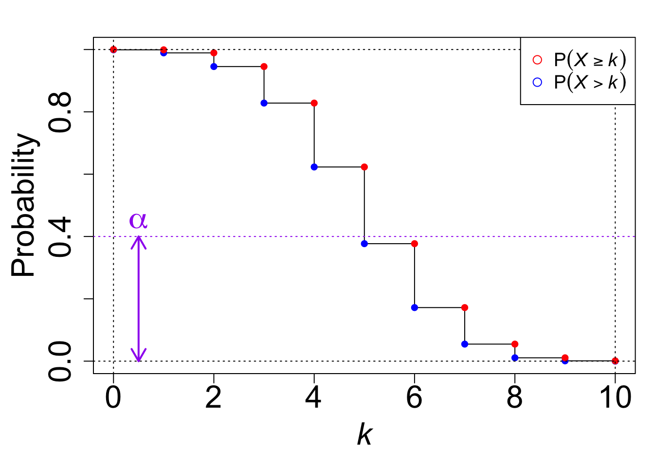
For this exercise, let’s consider a right-sided test. (Why? Because I had already made all the figures and schematics for a right-sided test before writing the last post, and don’t want to remake them for the left-sided test!) Again, consider the case of performing a hypothesis test \[\begin{aligned} H_{0} &: p \leq p_{0} \\ H_{1} &: p > p_{0}\end{aligned}\] for a binomial proportion (p) using a binomial random variable (X (n, p)). The classical right-sided (P)-value is then \[P = P_{p_{0}}(X \geq x_{\mathrm{obs}}).\] We know that this will, generally, be slightly too small at a boundary value of (x_{}): the difference between the largest (P)-value less than or equal to () and () will be non-zero unless we happen to have a “nice” sample size where that (P)-value is close to (). But we also know that (P_{p_{0}}(X > x_{})) will be slightly too big, since this is the first (P)-value that is stricly greater than (). The idea of a randomized (P)-value is to add a little fuzz to the classical right-sided (P)-value that will place us somewhere between (P_{p_{0}}(X x_{})) and (P_{p_{0}}(X > x_{})). That is, the randomized (P)-value is \[P_{\mathrm{rand}} = P_{p_{0}}(X > x_{\mathrm{obs}}) + U \times P_{p_{0}}(X = x_{\mathrm{obs}})\] where (U) is a uniform random variable on ((0, 1)) that is independent of (X).

Why does this work? Consider the sketch below, which shows the survival function (S(k) = P(X > k)) and its left-continuous analog (S(k^{-}) = P(X k)):

n <- 10
p <- 0.5

alpha = 0.4

ns <- 0:n

Ss <- pbinom(ns, n, p, lower.tail = FALSE)

par(mar=c(5,5,2,1), cex.lab = 2, cex.axis = 2)
plot(ns, Ss, type = 's',
     xlab = expression(italic(k)), ylab = 'Probability')

Ss.p1 <- Ss + dbinom(ns, n, p)
points(ns, Ss, col = 'blue', pch = 16)
lines(ns, Ss.p1, col = 'red', type = 'p', pch = 16)

abline(h = alpha, lty = 3, col = 'purple')
abline(h = c(0, 1), lty = 3)
abline(v = c(0, n), lty = 3)

legend('topright', legend = c(expression(P(italic(X) >= italic(k))),
                              expression(P(italic(X) > italic(k)))),
       col = c('red', 'blue'), pch = 1, cex = 1.2)

arrows(0.5, 0, 0.5, alpha, code = 3, col = 'purple', lwd = 2, length = 0.15)
text(x = 0.5, y = alpha+0.05, labels = expression(alpha), col = 'purple', cex = 2)

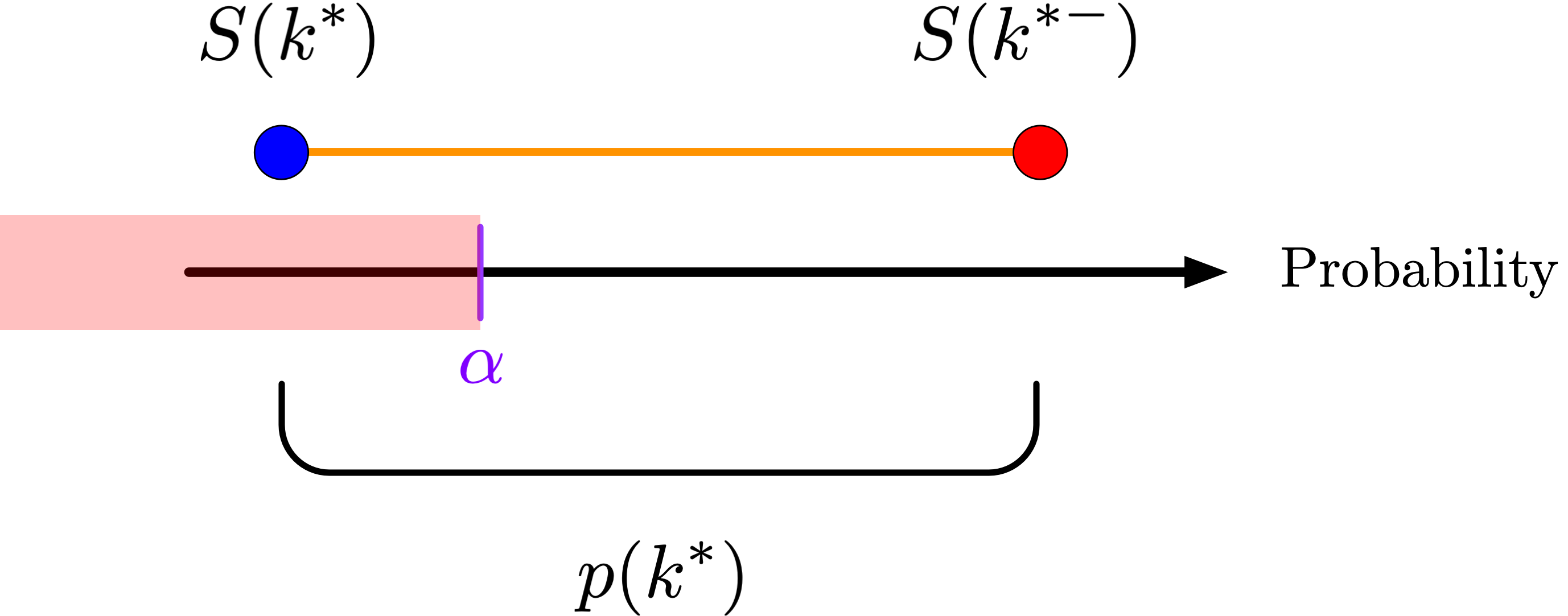
Here, (S(k^{-})) is the classical (P)-value, (S(k)) is the “too large” (P)-value, and the randomized (P)-value interpolates (randomly) between the classical (P)-value and the too small (P)-value: \[\begin{aligned} P_{\mathrm{rand}} &= P_{p_{0}}(X > x_{\mathrm{obs}}) + U \times P_{p_{0}}(X = x_{\mathrm{obs}}) \\ &= (1 - U) \times P_{p_{0}}(X > x_{\mathrm{obs}}) + U \times P_{p_{0}}(X \geq x_{\mathrm{obs}}) \\ &= (1-U) S(x_{\mathrm{obs}}) + U S(x_{\mathrm{obs}}^{-}). \end{aligned}\] The only place where the randomization has any effect occurs where the interpolating line crosses (); otherwise, anywhere we lie on the interpolating line we come to the same decision. Let (k^{}) be the first (k) such that (P(X > k) ). For (x_{} < k^{}), we fail to reject (H_{0}) and for (x_{} > k^{}), we reject (H_{0}). When (x_{} = k^{}), we use the randomization device. We should only reject when the randomized (P)-value is less than or equal to (), and hence when we fall in the portion of the interpolating line that is less than or equal to (). Rotating the figure above 90º counterclockwise, we have

and we should only reject when the (P)-value falls at or below (). Because (U) is uniform, the probability that this occurs is \[P\left(U \leq \frac{\alpha - S(k^{*})}{p(k^{*})} \right) = \frac{\alpha - S(k^{*})}{p(k^{*})}.\] So on the boundary of the rejection region, we reject (H_{0}) with probability (). Let ((X)) be our rejection rule, i.e. the function that is 1 when we reject the null hypothesis and 0 otherwise. Then () is a random function with the conditional distribution \[P(\phi(X) = 1 \mid X = k) = \begin{cases} 0 &: k < k^{*} \\ \frac{\alpha - S(k^{*})}{p(k^{*})} &: k = k^{*} \\ 1 &: k > k^{*} \end{cases}.\] Given this definition, it’s straightforward to prove that the probability that we reject the null hypothesis, that is, that ((X) = 1), is in fact (): \[\begin{aligned} P(\phi(X) = 1) &= \sum_{k} P(\phi(X) = 1 \mid X = k) P(X = k) \\ &= \sum_{\{k : k < k^{*}\}} 0 \cdot p(k) + \frac{\alpha - S(k^{*})}{p(k^{*})} p(k^{*}) + \sum_{\{k : k > k^{*}\}} 1 \cdot p(k) \\ &= \alpha - S(k^{*}) + S(k^{*}) \\ &= \alpha,\end{aligned}\] just as we wanted.

So a little uncertainty at the end buys us back our size, and we attain the desired significance level.