How to Burn Money and Computing Power for a Simple Median

NOTE: This is a parody post. It was generated by providing my code to GPT-4 with the prompt:

Turn this into a blog post with the title "World's Most Expensive Way to Compute a Mean or Median"

and then asking GPT-4 to make its initial post even more entertaining and sarcastic.

Introduction

Today, we dive into the comedic world of absurdly over-engineered solutions for simple problems. Our target? Calculating a mean or median using R and TensorFlow in what might be the most hilariously unnecessary method ever conceived.

Overkill Environment Setup

First things first: setting up our R environment. Sure, we could go easy with dplyr and ggplot2, but where’s the fun in that? Instead, let’s summon the computational titans - keras and tensorflow. Because obviously, when you think of finding a median, you think of deep learning, right?

library(dplyr)
library(ggplot2)

Sys.setenv(TF_USE_LEGACY_KERAS = 1L)
reticulate::use_python("/Users/daviddarmon/conda/envs/keras-legacy/bin/python")
library(keras)
library(tensorflow)

Creating a Monster Dataset

We’re cooking up a dataset y with 10,000 log-normally distributed random numbers. Normally, a simple task, but not today, folks. Today, we go big.

n <- 10000
y <- rlnorm(n)
x <- as.matrix(rep(1, n))

Frankenstein’s Neural Network

Now for the pièce de résistance: a neural network model using Keras, which is like using a sledgehammer to crack a nut:

u_per_h <- 5
H <- 10
activation <- "tanh"

model <- keras_model_sequential(input_shape = c(1L))

for (h in seq_len(H)) {
  model %>%
    layer_dense(units = u_per_h, activation = activation)
}

model %>%
  layer_dense(units = 1, activation = NULL)

model

Model: "sequential"
________________________________________________________________________________
 Layer (type)                       Output Shape                    Param #     
================================================================================
 dense (Dense)                      (None, 5)                       10          
 dense_1 (Dense)                    (None, 5)                       30          
 dense_2 (Dense)                    (None, 5)                       30          
 dense_3 (Dense)                    (None, 5)                       30          
 dense_4 (Dense)                    (None, 5)                       30          
 dense_5 (Dense)                    (None, 5)                       30          
 dense_6 (Dense)                    (None, 5)                       30          
 dense_7 (Dense)                    (None, 5)                       30          
 dense_8 (Dense)                    (None, 5)                       30          
 dense_9 (Dense)                    (None, 5)                       30          
 dense_10 (Dense)                   (None, 1)                       6           
================================================================================
Total params: 286 (1.12 KB)
Trainable params: 286 (1.12 KB)
Non-trainable params: 0 (0.00 Byte)
________________________________________________________________________________

286 parameters to memorize 1 number!

Training: Because We Can

Let’s train this beast. Our loss function? Mean Absolute Error (MAE). Our optimizer? Stochastic Gradient Descent, because why make it easy?

loss <- "mae"

model %>%
  compile(
    loss = loss,
    optimizer = optimizer_sgd(learning_rate = 0.03)
  )

Training involves a batch size equal to the length of x, 200 epochs, a 20% validation split, and early stopping to pretend we care about efficiency.

history <- model %>%
  fit(
    x, y,
    batch_size = nrow(x),
    epochs = 200,
    validation_split = 0.2,
    callbacks = callback_early_stopping(patience = 10, restore_best_weights = TRUE)
  )

plot(history, smooth = FALSE) +
  theme_bw() +
  theme(text = element_text(size = 20))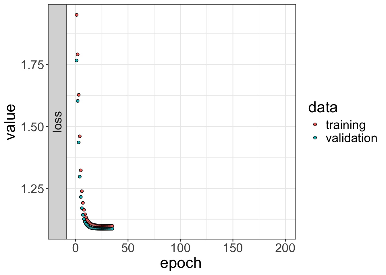

The Grand Reveal

At last, let’s compare the good old-fashioned mean and median with our neural network’s predictions:

loss

[1] "mae"

mean(y)

[1] 1.627241

median(y)

[1] 1.011186

predict(model, x) %>% head(1)

313/313 - 1s - 630ms/epoch - 2ms/step

          [,1]
[1,] 0.9778503

Conclusion

Our journey through the world of computational overkill serves as a hilarious, yet poignant, reminder: sometimes, the simplest tools are the best. This laughably complex method for computing a mean or median underscores the value of choosing the right tool for the task at hand in data analysis. Remember, folks, sometimes less is more!